One of the best ways to organize references across complicated Excel tables is by using structured references. They are related to Tables and directly refer to cells, rows, columns of Tables or the combination of these without having to use cell coordinates. In simple terms, they turn references like “A2:B6” into descriptive ones where it’s easy to instantly see their purpose, like “Table[January]” or “[@January]:[@February]”.
Using structured references keeps your Excel functions tidy and makes them more resilient to data changes. With proper table references, changing source data needs no formula updates.
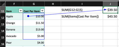
Before adding the item “Pear”, both functions calculated the same amount. Adding a new item at the bottom of the table (Pear) the SUM functions referring to the cells above aren’t updated to include it. The second function that directly refers to the table column needs no updates, it shows the correct amount as the table is extended.
Creating table references in Excel
Just like simple cell references you can easily create them by selecting the appropriate table range with the mouse or typing it using their special syntax. It’s important that they only work in tables, so data should first be converted into a table by either selecting “Format as Table” from the Home ribbon or simply pressing Control-T (Cmd+T on a Mac).
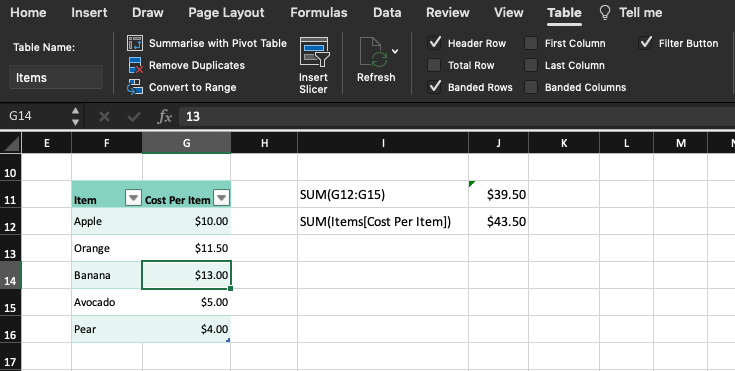
Each table should have a unique name that can be changed in the Table ribbon together with various other options. Pick a short, descriptive name so functions with references in them will be easy to understand. A reference within the same table will normally leave out the table name, e.g. “Items[Cost Per Item]” simply becomes [Cost Per Item].
Structured reference format
The simplest syntax to refer to tables in Excel functions is Tablename[ColumnName], where ColumnName refers to the data part of the column. There are a few special identifiers that can be used instead of column names, they all start with a pound sign.
A reference consists of three things, the Table name, the Item specifier, and a Column specifier.
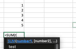
Excel helpfully displays a tooltip and auto-completes all possible options, when creating a new reference. It’s a great way to experiment with various options and explore the possible reference combinations:
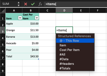
- #All – refers to the whole table, in this example A1:B7
- #Data is the data part, A2:B7
- #Headers is the row containing column headers, A1:B1
- #Totals is the bottom row listing totals, A7:B7
Data columns can simply be referenced by the column name (without quotes), for example Items[Item].
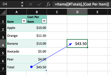
When referring to specific parts of a column, for example, the Totals row of the Cost Per Item column, the following format should be used: Items[[#Totals],[Cost Per Item]]. In this example #Totals is the column specifier and “Cost Per Item” is the item specifier.
The current row can be referenced by using the “@” sign, this is mostly useful when adding functions with structured references to a column inside the table itself. When a function refers to a cell or a range inside table, the table name can be omitted, so for example =[@Item] refers to the cell in the Item column and the same row as the function itself.
Reference range operators
There are three reference operators that are useful with structured ranges, the colon, the command, and the space. They can be used to combine ranges in column specifiers, similarly to simple ranges. When a column specifier contains operators, each column range should be enclosed in square brackets.
The colon (range) operator combines parts of adjacent ranges including everything in between them, Items[[Item]:[Cost Per Item]] refers to the data range of both columns, A2:B6
The comma (union) operator combines all the ranges separated by commas without including the cells between those ranges. In our case, Items[Item], Items[Cost Per Item] is the same as Items[[Item]:[Cost Per Item]] because there are no columns between the two.
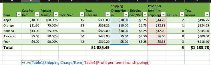
The space (intersection) operator calculates the overlapping parts of two ranges. In the example above, the Total Revenue cell can be referenced using Table1[[#All],[Total Revenue]] Table1[#Totals], intersecting the Totals column and the Total Revenue row. In this case, it’s equivalent to Table1[[#Totals],[Total]
Tips using structured references in Excel
When you work with table references in Excel, there are a few simple ways to create a reference to them by using either the keyboard or the mouse. Most of the time the simplest way to experiment with them is to simply start creating a new function in an empty cell by typing “=” then using the mouse to select various parts of the table to see how the reference changes. You can exit this mode by simply pressing the ESC key.
Autocomplete is another useful feature that helps to create structured references, a dropdown menu is automatically displayed showing all the possible options, then TAB autocompletes and copies the first possible option into the cell. For example to quickly create a function in a cell that displays the sum of all the items sold with the keyboard only (=SUM(Table1[Total Sold]), you would type keys in the following order:
=SUM(Ta <TAB> [To <TAB> ])Every time the <TAB> key is pressed, it automatically enters the first possible option in the dropdown. Cursor arrow keys can be used to select different options then <TAB> copies them into the new function.
It’s useful to name tables, rows, columns in a short but descriptive way so they are easy to use in references. Spaces can be added to formulas to make them more readable, this is especially convenient in complicated formulas containing multiple references with commas.
Named ranges
There maybe be cases when converting data into tables is simply not suitable for the data format. Excel provides another tool to simulate structured range references in these cases, by using named ranges.
They can be created by simply selecting a range of cells in a workbook then either pressing CTRL+F3 (CMD+F3 on a mac) or selecting “Define Name” from the Formulas ribbon.
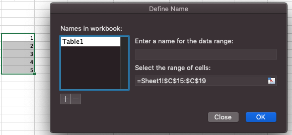
Here you can create a named range by simply entering a new name into the name field, then pressing Enter or clicking the OK button.
Once a named range is created, it works similarly to structured references, autocomplete works and they are treated just like table names and they can be used in formulas by simply typing the name of the range instead of cell references.