Dropdown lists are a great way to allow a user to pick a cell value from a list of possible options. Excel provides combobox style dropdown lists, input validation tools, and error messages to customize the user experience.
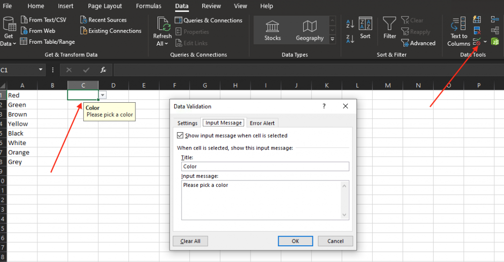
This option is accessible in the “Data” ribbon in the “Data Tools” group or in the Data > Validation menu.
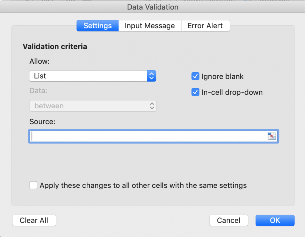
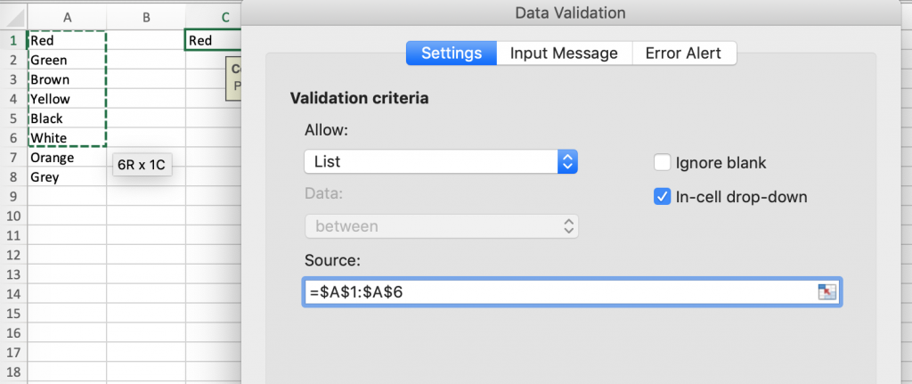
When “List” is selected from the possible data validation choices, the active cell becomes a Drop-down list. The Source field is mandatory, it defines the list of possible options.
Basic Data Validation sources
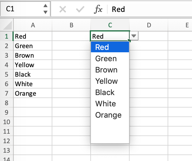
Let’s make a list of Colors in the A column, then select the C1 column and activate Data Validation. Clicking Source, then clicking the “A” column header will enter “=$A:$A” in the Source field, making the source of the dropdown the whole A column.
This instantly creates a simple dropdown in cell C1, showing as a dropdown menu. Its values are limited to the ones in column A as shown below:
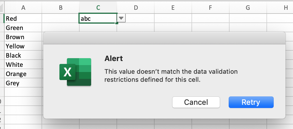
The advantage of this is that adding any elements to column A automatically shows up in the list of possible options in the dropdown cell. Typing an invalid value results in an error message showing that the value fails data validation,
Direct data references
Instead of selecting a range of cells as a list of possible options, it’s also possible to type directly into the Source field and list options, separated by a comma. For example, typing “Yes, No, Maybe” will create a dropdown with three options: Yes, No, and Maybe
Customizing error messages
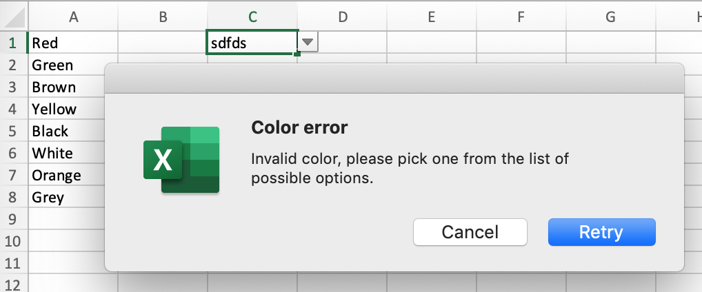
Whenever a bad valid is entered in the cell, clicking “out” of the cell or pressing Enter instantly shows an error message. Under the Error Alert tab of the Data Validation window, you can customize the error message dialog.
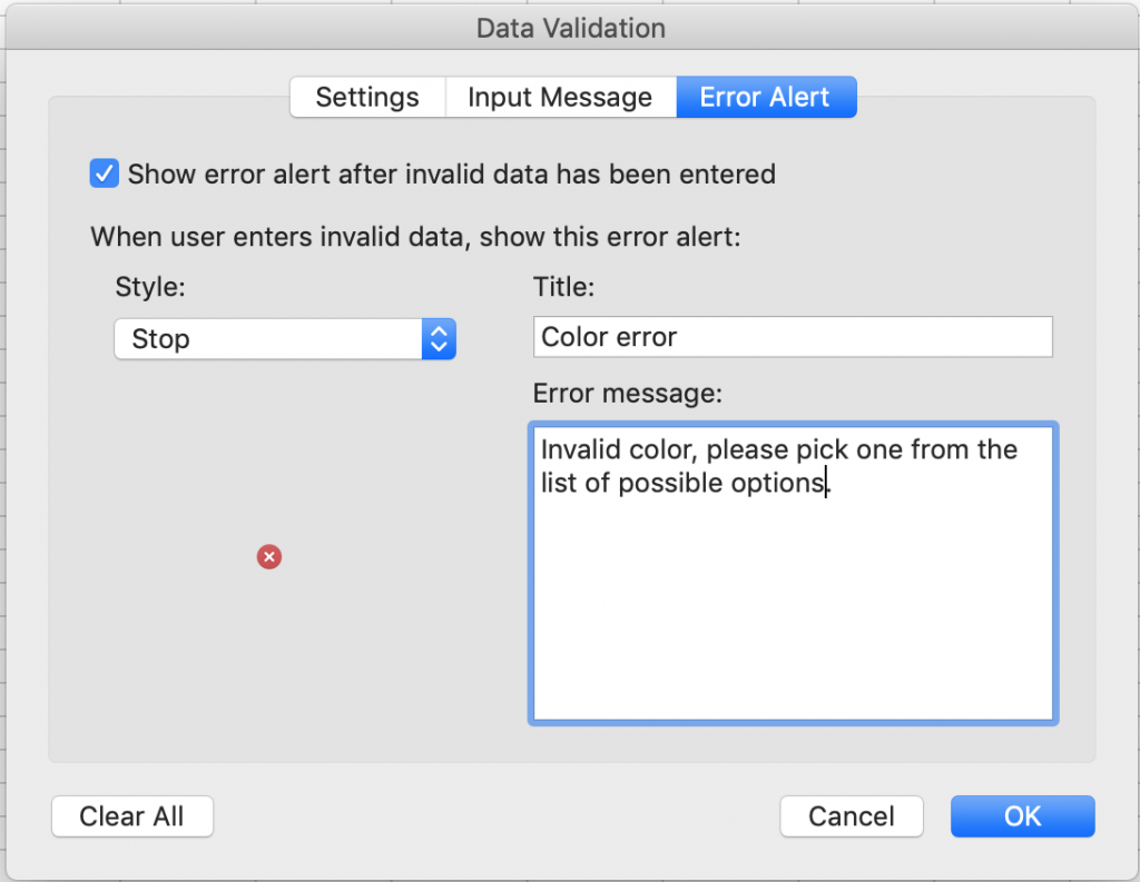
It has three properties, Style, Title, and the Error Message itself. Style defines the basic style of the dialog (Error / Warning / Information). Title sets the title of the error message dialog and “Error message” sets the message itself to be displayed.
Unchecking the Show error checkbox on top will disable validation while keeping the dropdown operational, so no error will be shown if the entered data is invalid.
Adding an input message to the dropdown menu
To better explain to the user what the cell dropdown is about, you can also add extra instructions that show up when the cell is activated. The functionality is contained in the Input Message tab of the data validation window. You can set the Title and the input message and it shows as a tooltip when the cell is active.
Removing a dropdown list
To remove a dropdown list, simply open the Data Validation popup again and set the validation criteria back to their default setting: any value. It will remove the dropdown from the cell, leaving you with the last entered value without the dropdown functionality.
Using named ranges in drop-downs
So far we have looked at two ways to define the possible options for the drop-down cells. We could either define them directly by setting the “Source” field to a comma-separated values, or set it to a whole column. It’s also possible to set it to a range, by simply manually selecting the range after clicking on the Source field:
Defining a named range makes it a lot easier to keep track of range references, especially when the worksheet structure becomes too complicated – it’s also easy to simply modify the range and update all references including drop-down cells – they will get updated automatically to reflect the change in the named range. If you’re interested in named ranges and Excel structured references in general, you can find more information about them here: Excel structured references explained.
To define a named range, first select all the cells (in our case all the colors in column A) then open the name manager by clicking “Define name” in the Formulas ribbon.
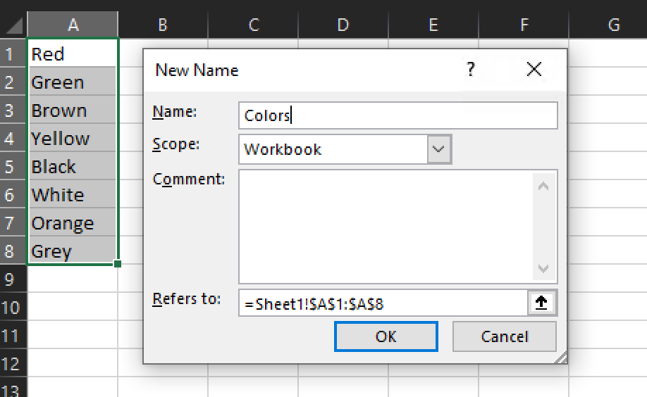
You’ll need to change the Name (by default it sets the name to the first cell, in our case: Red) and leave the rest of the settings to defaults. The Scope defines the visibility of the Names range, Workbook means that every sheet in the same workbook can reference this range.
Once the range is defined, it becomes possible to simply reference this range (Colors) in the Data Validation popup, by setting the Source to “=Colors” (without quotes). Excel is also smart to automatically replace the range to its Names range counterpart if all the cells in the range are selected.
Creating dependent drop-downs
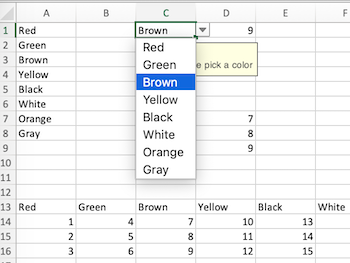
By using formulas as the dropdown source value, it’s possible to create dependent dropdowns. For example, let’s create a second dropdown where its validation options should depend on the selected value of the first column.
To achieve this, we need to define a formula that returns an array depending on the value of the first dropdown and set it as the source of the second dropdown in its Data Validation popup.
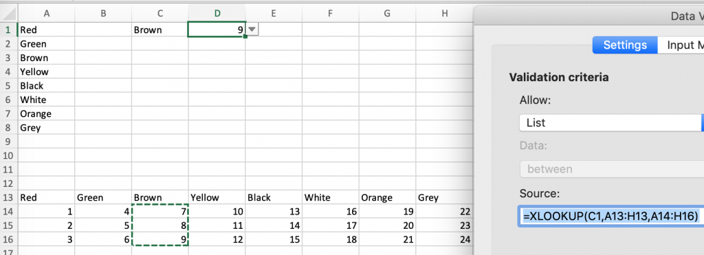
Here, the XLOOKUP formula takes the value of the first dropdown cell (C1), finds it in the range A13:H13 (the horizontal list of colors), then returns the appropriate range just below the matched color. This way, selecting “brown” for example, will find it in C13 and return the list “7,8,9” in the cells just below it.
It is possible to use pretty much any function to generate the list of options for validation, so the second dropdown validation and its list of options will depend on the cells the function in the “Source” setting refers to.
Removing empty values
The example above exploits the fact that all possible dependent options have three values below them, so a simple XLOOKUP returns the right amount of information. If we were to have an arbitrary number of options under each color, we could extend the range to include all of them, however, colors with fewer options would display a few empty options. The same issue appears if the named range has some “holes” in them – cells with empty values.
The FILTER function is a great way to remove empties – it can remove values from an array that fulfill specific criteria, in our case the ones that are empty. Instead of the previous function:
XLOOKUP(C1,A13:H13,A14:H17)we need to use this:
=FILTER(XLOOKUP(C1,A13:H13,A14:H17),NOT(ISBLANK(XLOOKUP(C1,A13:H13,A14:H17))))or its shorter equivalent:
=FILTER(XLOOKUP(C1,A13:H13,A14:H17),""<>XLOOKUP(C1,A13:H13,A14:H17))The FILTER function requires two arrays, one is the array it will filter, the second one is an array of logical values that tell whether the element from the first array should be included. So, for example, the function
=FILTER({1,2,3},{FALSE,TRUE,TRUE})will return 2,3, because the first element of the second array is false but the rest of them are true.
This technique is useful when you need to remove blanks from a list of values so in handy when creating dynamic dropdown lists.